This guide has been written to outline the key steps need to create a number of reports and while the examples have been written against demonstration retail data, the methodology is easily transferable to other data sets.

When creating a report, the preview at the bottom of the screen will reflect the current layout of the report against a limited number of records. Clicking this preview will also reveal styling options to tailor the reporting output.

Basic Reports

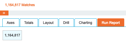
When the Crosstab functionality is initially accessed, the default Total Type is set to Count, where a simple record count is performed. This can be verified by clicking Run Report with no options set, where the report will simply display number of records:

When creating Crosstab reports, it is important to remember that fields that require aggregations should not be used as rows or columns and should instead be created as totals. With more than one total and only rows specified as the axis, the totals effectively become the columns.

Report Containing a Single Row and Single Total

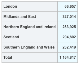
The following report displays the number of transactions by Region Name:

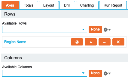
This has been created by selecting a single Row in the Axes tab:

A single total with the default Count Total Type was used:

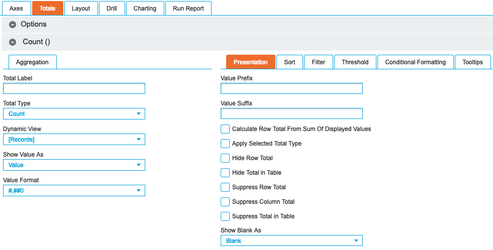
As the Total Label has been left blank, the total has been automatically named ‘Count()’. While this does not have any meaningful impact on this simple report, labelling totals will simplify the management of more complex reports.

Report Containing Multiple Rows in Sorted, Filtered Groups

This report displays the top 5 sales within a grouping hierarchy drillable by Product Department and Product Group, notice that the number of sales for these 5 results are a subset of International Cuisine's total:

The report has been created using Rows 'Product Department', 'Product Group' and 'Product Name', in the Axes tab:

Row settings have been changed to Drillable Hierarchy with Row Axis Labels & Show Row Numbers both enabled.

A single total with the default Count Total Type was used. Sort > Row Sort has been set to Descending and Filter > Filter has been set to Top Value with Type of Cell and Filter Value to 5:

Report Containing Single Column and Single Total

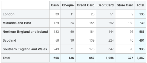
The following report displays the number of transactions for each method of payment:

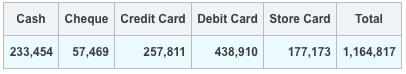
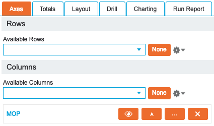
This has been created by selecting a single Column in the Axes tab:

A single total with the default Count Total Type was used, as detailed in the previous example.

Report Containing Basic Total

Creating reports that contain basic totals, such as Average or Sum, is a very simple task that can be created on an ad hoc basis using a number of user-friendly drop-down lists.

The following report displays the average basket value for each region:

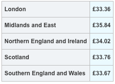
This has been created by selecting a single Row in the Axes tab:

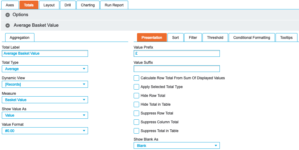
A single total with the Total Type set to Average has been used. Once the Total Type has been set to anything other than Count or Calculation, the Measure drop-down list becomes available, where the fields available to use in totals are displayed. If the required fields do not appear in this list, please contact the system administrator.

In this example, the Value Format has been set to #0.00 and a Value Prefix of £ has been added to denote monetary value:

Finally, the column total has been hidden as it does not display meaningful information when returning averages in the report. This is achieved by clicking the Cog icon in the Axes tab in the Columns section and selecting Column Totals Hidden:

Report Containing Standard Calculation

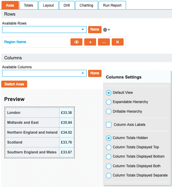
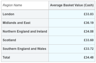
The following report displays the average basket value for cash transactions against each region:

This has been created by selecting a single Row in the Axes tab:

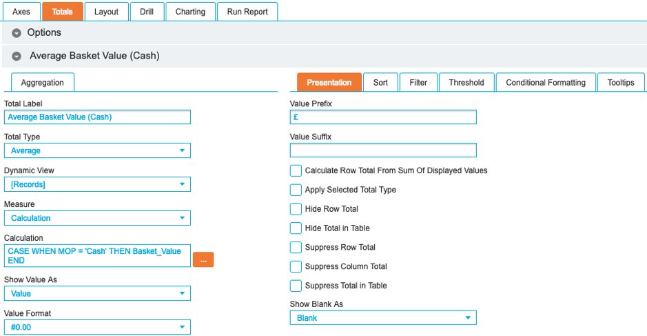
As with the previously detailed report, the Total Type has been set to Average. However, rather than selecting a field from the Measure drop-down list, select Calculation.

Once Calculation has been selected, click …  to open the Calculation Builder. Add the following:

CASE WHEN MOP = 'Cash' THEN Basket_Value END

A standard calculation will perform the statement on a row-by-row basis. For each row, the MOP (method of payment) field is scanned for the value ‘Cash’. When true, the Basket Value value is stored. Once the calculation has been run against every row, the Average Total Type is applied.

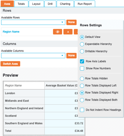
Finally, the row axis labels have been enabled to add headers onto the report. This is achieved by clicking the Cog icon in the Axes tab in the Rows section and enabling Row Axis Labels:

Report Containing Cell Calculation

Cell Calculations behave very differently to Standard Calculations.

Rather than apply the calculation on a row-by-row basis, values from existing totals are used, permitting the use of pre-aggregated values in calculations.

A Cell Calculation can only be performed when at least one other total has been created in the report.

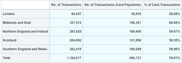
The following report displays the total number of transactions, the number of transactions paid via card and the percentage of transactions paid via card per region:

This has been created by selecting a single Row in the Axes tab:

Multiple totals have then been created.

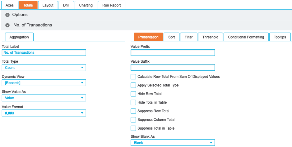
The first total has the Total Type set to Count and has been labelled ‘No. of Transactions’:

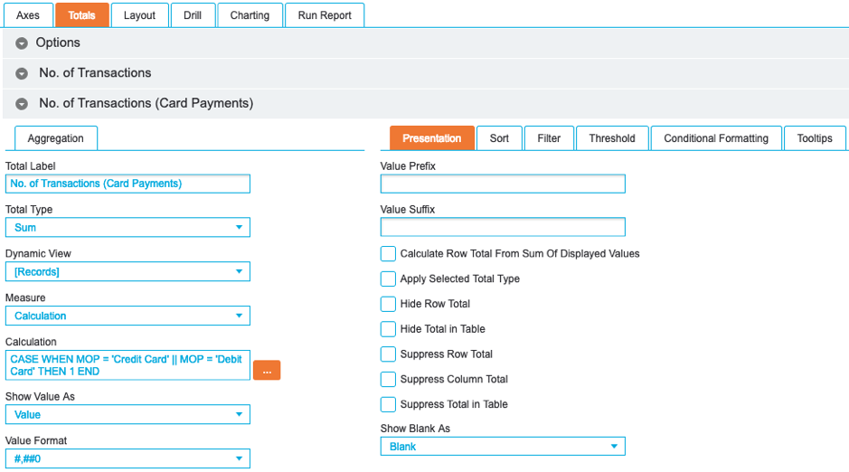
The second total has been labelled ‘No. of Transactions (Card Payments)’ with the Total Type set to Sum, as each row needs to be added up, and the following calculation logic applied:

CASE WHEN MOP = 'Credit Card' || MOP = 'Debit Card' THEN 1 END

Using two pipes (||) in the calculation performs the OR function, permitting more than one value to be specified. In this instance, both ‘Credit Card’ and ‘Debit Card’ values are of interest to represent all card-based transactions:

The third total, labelled ‘% of Card Transactions’, has the Total Type set to calculation and the following calculation logic applied:

'No. of Transactions (Card Payments)'/'No. of Transactions'*100

This logic calculates the percentage value from the two previously created totals. Please note that calculations are handled sequentially when the Run Report tab is clicked. This means that the first two totals must run before the Cell Calculation.

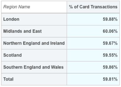
This report can be taken a step further by hiding the first two totals and only displaying the percentage value. Simply enable the Hide Row Total option for the first two totals and enable the Row Axis Labels option in the Axes screen. This will display the following report, where the underlying logic for all three totals is still present, but only the Cell Calculation total value is displayed:

Report Containing DrillThru

For calculations in a report, users are not able to drill through to the underlying records without translating the calculation logic into syntax that can be parsed in the Query screen.

To ensure that users navigate to the correct underlying values, the DrillThru value is used in calculations.

The following report displays the number of cash transactions per region:

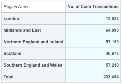
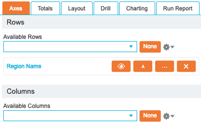
This has been created by selecting a single Row in the Axes tab and enabling the Row Axis Labels setting:

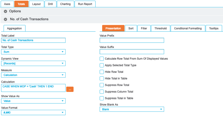
A single total has been created, labelled ‘No. of Cash Transactions’, with the Total Type set to Sum, the Value Format set to Sum, the Value Format set to #,##0 and the following calculation logic applied:

CASE WHEN MOP = 'Cash' THEN 1 END

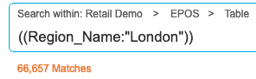
When this report is run and a value is clicked, notice how the generated query does not factor in the calculation when drilling through to the underlying records:

Amend the calculation to the following:

CASE WHEN MOP = 'Cash' THEN DrillThru(1) END

The following query is now generated when clicking the same value in the report:

When the calculation logic is wrapped in the DrillThru value, it can then be translated to the required query syntax. In this example the ‘1’ value represents the calculation logic, instructing the total to include the rows in the sum.

Report Referencing Specific Cells

The following report displays the number of transactions for each method of payment by region. It also includes a cell/Total Calculation called ‘Central and East Store Cards’ which demonstrates the row and column reference functions which include results of both the London & Midlands and East region's store card sales:

You will notice that due to referencing specific cells from the crosstab, the context is independent of the row/column axis. This is done using the cell/Total Calculation formula below:

Sum(rows('London'),columns('Store Card'),0)
+
Sum(rows('Midlands and East'),columns('Store Card'),0)

With Region Name selected as a single Row with totals hidden selected under the row settings, and MOP as the column in the Axes tab:

MOP values selected in the column axis are 'Cash' & 'Store Card' to filter down to just these results:

In the Totals tab, 'No of Transactions' is entered using the Total Type set to the default Count option. The cell/Total Calculation formula mentioned above can be entered in the calculation box and labelled as 'Central and East Store Cards':

Report Referencing Min/Max Column Totals

The following report displays the number of transactions for each method of payment by region. It also includes two cell/Total Calculations called 'Region Minimum' & ‘Region Maximum’ which demonstrates the ColumnMin() and ColumnMax() reference functions:

You will notice that due to referencing min & max column values from the crosstab, the context is independent of the row/column axis. This is done using the cell/Total Calculation formulas below:

ColumnMin( 'No. of Transactions' )
ColumnMax( 'No. of Transactions' )

With Region Name selected as a single Row with totals hidden selected under the row settings, and MOP as the column in the Axes tab:

MOP values selected in the column axis are 'Cash' & 'Store Card' to filter down to just these results:

In the Totals tab, 'No. of Transactions' is entered using the Total Type set to the default Count option. The cell/Total Calculation formulas mentioned above can be entered in the calculation box and labelled as 'Region Minimum' & ‘Region Maximum' respectively:

Variance Reports

Variance reports are a common reporting requirement and are often used for comparing period-to-period or year-to-year sales.

Report that Compares Sales

The following report compares the variance between the regional sales for the previous year compared to the current year, then changes the text colour based on an increase or decrease in sales. The Current Year figure is red if the total is less than the previous year, and green if the total is more than the previous year:

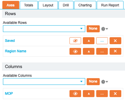
This has been created by selecting a single Row in the Axes tab:

Multiple totals were then created.

The first total has been labelled ‘Previous Year Sales’ with the Total Type set to Sum, the Value Format set to #,##0.00, a Value Prefix of £, the Hide Row Total and Hide Total in Table options enabled and the following calculation logic applied:

CASE WHEN ToYear(Transaction_Date) =  ToYear(TODAY) -1 THEN Line_Price END

For each row, this will extract the year from the Transaction Date field and determine if it matches the current year when the report is run, denoted by ‘TODAY’, minus one year. When matching, the Line Price is added to the total.

Clicking the Copy icon for a total will create an exact copy below. This is especially useful when the display options, such as Value Format, have already been set.

The second total has been labelled ‘Current Year Sales’ with the Total Type set to Sum, the Value Format set to #,##0.00, a Value Prefix of £ and the following calculation logic applied:

CASE WHEN ToYear(Transaction_Date) =  ToYear(TODAY) THEN Line_Price END

This uses the same methodology as the previous total, but does not hide the output and only adds the Line Price value to the sum when the year part of the Transaction Date field matches the current year when the report is run.

The third total is a Cell Calculation labelled ‘Variance’ with the Total Type set to Calculation, the Value Format set to #,##0, a Value Suffix of %, the Hide Row Total and Hide Total in Table options enabled and the following calculation logic applied:

('Current Year Sales'/'Previous Year Sales')*100

This divides the second total value from the first and multiplies the output by one hundred to derive the variance percentage value.

This total will not be displayed in the final output. Instead, the values will be used to drive the conditional formatting for the 'Current Year Sales' total.

In the Conditional Formatting tab of the 'Current Year Sales' total, the Source Value drop-down list controls the total value that will be used. By default, this will be set to the current total.

In this example, the 'Variance' total has been selected from the Source Value drop-down list for two conditions. The first condition will change the the text colour to red when the total is less than 100, while the second condition will change the text colour to green when the total is greater than or equal to 100.

Finally, the Scope drop-down list controls which portion of the report will be styled based on when the conditions are met. In this example, Row Totals Displayed has been selected.

Row Total Reports

For reports that require a separate total for each row, Row Totals are used.

In most cases, reports that use Row Totals will use placeholders as axis to structure the output rather than actual fields from the Index. Placeholders act as row labels that do not perform any filtering, with this instead handled at calculation level.

Report Containing Row Totals

The following report displays a summary of key metrics across the different regions:

This has been created by selecting the Saved entry for the Row and a single entry for the Column in the Axes tab:

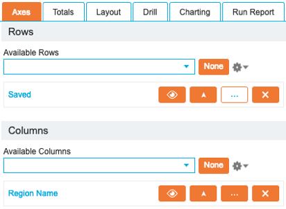
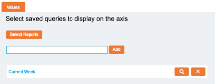
The Saved entry, located at the bottom of the list, allows placeholder values to be added to the report. Click the … button for the saved entry to display the Values popup. Enter the name of the required placeholder in the textbox and click Add to save the entry. Click Apply to complete the process.

Multiple row totals were then created.

With the Total Type drop-down list set to Row Total, the Measure drop-down list will automatically select Row Total Calculations. The drop-down list below can then be used to select each row that will be used in the report.

With the rows selected, a separate calculation can now be written against each entry. Click the … icon for each row to specify the logic that will be used:

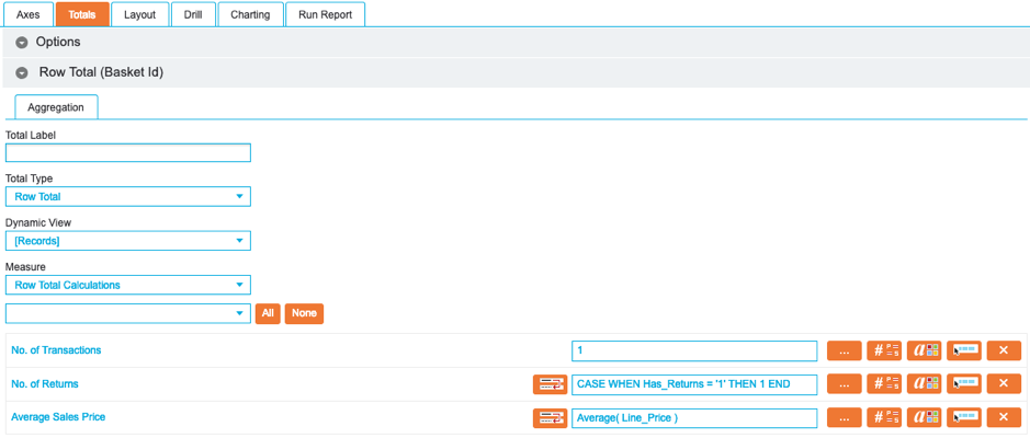
The first total for the ‘No. of Transactions’ row simply uses 1 as the calculation logic. This provides a row count, which represents the total number of transactions in the Index.

The second total for ‘No. of Returns’ uses the following logic:

CASE WHEN Has_Returns = '1' THEN 1 END

For every row, the Has_Returns field is scanned for the value ‘1’. When true, the row is added to the row count that will represent the number of returned items in the Index.

Finally, third total for ‘Average Sale Price’ uses the following logic:

Average( Line_Price )

This simply averages the Line_Price value for every row. More mathematical functions can be found in the Calculation Builder Functions drop-down list.

As the first two totals are displaying row counts and the third total is displaying an average of monetary value, the Value Format will need to be different. When using row totals, this can be handled separately for each total via the Style icon:

For the third total, the Value Format and Prefix can then be set accordingly:

Finally, when creating row total reports, it is important to consider the validity of row and column totals. In this example, there are two row counts and an average monetary value – summing these values together will not produce any meaningful output. In this report, they will be hidden.

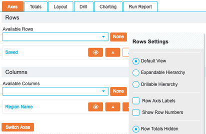
This is achieved by clicking the Cog icon in the Axes tab in the Rows section and clicking Row Totals Hidden:

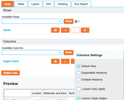
The same can be applied to the column totals by clicking Column Totals Hidden:

If the logic used does dictate that row or column totals are required, ensure that the Calculate Row Total From Sum of Displayed Values is enabled in the Totals tab. This will sum the on-screen values rather than taking the count from the unfiltered underlying Index.

Row Calculation Reports

Not to be confused with row totals, row calculations allow blank rows to be repurposed to contain calculations between other rows in a report.

Report Containing a Row Calculation

The following report displays the number of transactions for each method of payment. It also includes a row calculation called ‘Bank Card Sales’ which includes data from both debit card and credit card sales:

This has been created by selecting a single Row in the Axes tab:

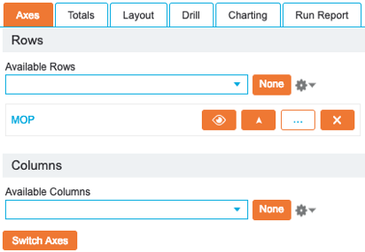
To add the new value to the report, click the … icon for the field and navigate to the Groups tab before creating a group for each individual value. In addition, create a blank group titled ‘Bank Card Sales’:

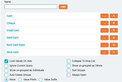
The default Crosstab behaviour is to hide rows that do not have any attached data. To override this behaviour and ensure that the empty row is displayed, enable the Lock Values On Axis option.

In the Totals tab, a new Row Calculations tab will now become available that allows a calculation to be written against the empty row:

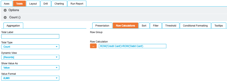
The following logic has been applied:

ROW('Credit Card')+ROW('Debit Card')

This will simply sum the output from both the ‘Credit Card’ and ‘Debit Card’ rows.

Formfield Calculation Reports

Using filters is an effective way to reduce the record count to a cohort of interest that not only focuses the output, but also optimises the loading time by reducing the number of records that are used in calculations.

Rather than filtering the data for the entire report, it is also possible to use filters as referenceable parameters.

Report Containing a Formfield Calculation

The following report displays the month-to-date (MTD), year-to-date (YTD) and last year’s month-to-date sales for each region:

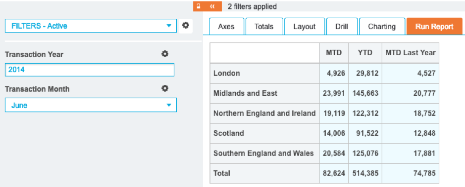
Despite the filters being set to June 2014, the use of formfield calculations results in the ‘YTD’ and ‘MTD Last Year’ totals not being filtered to only June 2014 data.

To produce this report, two filters named Transaction Year and Transaction Month are required. Importantly, the Ignore option must be enabled for each filter under the Advanced Options. This stops the filters having any effect on the report unless specified in a calculation.

The report has been created by selecting a single Row in the Axes tab:

Multiple totals have then been created.

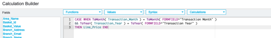
The first total has the Total Type set to Sum, Measure set to Calculation and has been labelled ‘MTD’. The following calculation logic has been applied:

CASE WHEN ToMonth( Transaction_Month ) = ToMonth( FORMFIELD^"Transaction Month" ) && ToYear( Transaction_Year ) = ToYear( FORMFIELD^"Transaction Year" ) THEN Line_Price END

In this statement, to define the month-to-date sales, every row is scanned to determine if the Transaction Month value matches Transaction Month filter and if the Transaction Year value matches the Transaction Year filter. These values are then summed and output into the report.

The FORMFILED^ syntax is used to reference filters in the calculation builder.

When referencing a filter using the FORMFIELD^ syntax, double quotes must be used.

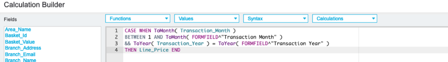
The second total has the Total Type set to Sum, Measure set to Calculation and has been labelled ‘YTD’. The following calculation logic has been applied:

CASE WHEN ToMonth( Transaction_Month ) BETWEEN 1 AND ToMonth( FORMFIELD^"Transaction Month" ) && ToYear( Transaction_Year ) = ToYear( FORMFIELD^"Transaction Year" ) THEN Line_Price END

In this statement, to define the year-to-date sales, every row is scanned to determine if the Transaction Month field is between January and the Transaction Month set in the Filter and if the Transaction Year field match.

The ToMonth function returns a numeric value (January = 1, February = 2 etc.) and the BETWEEN statement uses 1 (January) as the starting point of the range. These values are then summed and output into the report.

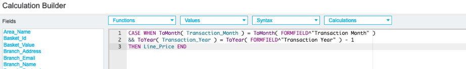
The third total has the Total Type set to Sum, Measure set to Calculation and has been labelled ‘MTD Last Year’. The following calculation logic has been applied:

CASE WHEN ToMonth( Transaction_Month ) = ToMonth( FORMFIELD^"Transaction Month" )
&& ToYear( Transaction_Year ) = ToYear( FORMFIELD^"Transaction Year" ) - 1
THEN Line_Price END

This statement uses the same logic as the first total, but importantly includes -1 after the ToYear syntax. This instructs the system to take the output and then display the results for the previous year.

Variance Report Containing a Formfield Calculation

The following report compares the average profit for a filtered date range against the whole dataset for each region and method of payment. The variance is then dynamically output to denote whether the filtered range value is greater than or less than the value across the entire Index:

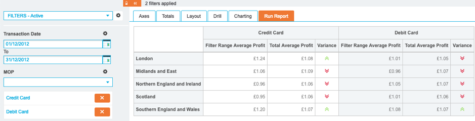
To produce this report, a date range filter named Transaction Date is required. Importantly, the Ignore option must be enabled for this filter under the Advanced Options. This allows end-users to select a custom range when running the report that only impacts the ‘Filter Range Average Profit’ total. A second droplist multi filter for MOP has been added to further focus the output.

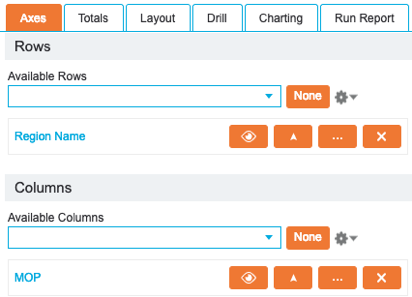
The report has been created by selecting a single Row and single Column in the Axes tab, with Row Totals Hidden and Column Totals Hidden selected from the corresponding Cog menu:

Multiple totals have then been created.

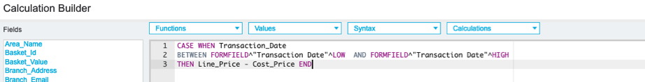
The first total has the Total Type set to Average, Measure set to Calculation and has been labelled ‘Filter Range Average Profit’. The following calculation logic has been applied:

CASE WHEN Transaction_Date BETWEEN FORMFIELD^"Transaction Date"^LOW  AND FORMFIELD^"Transaction Date"^HIGH THEN Line_Price - Cost_Price END

In this statement, the profit is derived for every transaction where the transaction date falls between the date range set in the filter panel. The profit is calculated by subtracting the cost price (the amount the product cost the business) from the line price (how much the product was sold for).

The FORMFIELD^"Transaction Date"^LOW logic refers to the from value in the range filter and the FORMFIELD^"Transaction Date"^HIGH’ logic refers to the to value in the range filter.

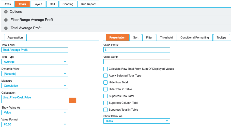
The second total has the Total Type set to average, Measure set to Calculation and has been labelled ‘Total Average Profit’. The following calculation logic has been applied:

Line_Price-Cost_Price

This calculates the profit value, as detailed for the previous calculation, for every row and averages the output. This total is not impacted by the Transaction Date filter, and instead provides a benchmark figure for every row of data that the filtered total can be compared against.

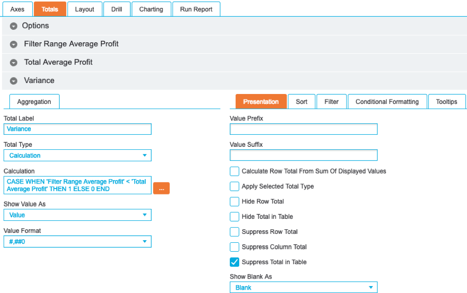
The third total has the Total Type set to Calculation and has been labelled ‘Variance’. The following calculation logic has been applied:

CASE WHEN 'Filter Range Average Profit' < 'Total Average Profit' THEN 1 ELSE 0 END

This cell calculation simply outputs a 1 when the first total is less than the second total, and a 0 when the opposite is true. These values provide the logic for the conditional formatting, and enabling the Suppress Total in Table option will hide the values:

Save the current report and import the following images:

In the Conditional Formatting tab for the third total, the following conditions can now be created:

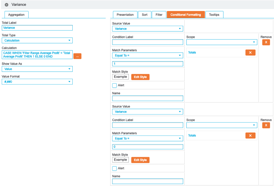
The first condition has been set to Equal to 1 and the Scope set to Totals. The Edit Style button can then be used to modify the output, where the Image option can be used to select the ‘Red Down Arrow’ image.

The second condition has been set to Equal to 0 and the Scope set to Totals. The Edit Style button can then be used to modify the output, where the Image option can be used to select the ‘Green Up Arrow’ image.

When end-users view the report and change the Transaction Date filter, the report will now dynamically output the corresponding image when the filtered value is greater than or less than the total average value. 

Saved Query Reports

Utilising the flexibility of saved queries in Crosstab reports provides a number of ways to output cohorts of interest to not only optimise the rendering time, but to maintain the integrity of a published report.

Report Using a Saved Query as a Hidden Filter

The following report displays the number of transactions that have been processed for the current week for each region and method of payment:

Rather than using a filter or the query bar the reduce the records, a hidden saved query has been used to drive the report at axis level. Due to the sequential nature of how a Crosstab report is run, the record count is reduced before any calculations are run, significantly optimising the render process. Furthermore, using queries in this manner maintains the integrity of the report as the syntax cannot be viewed or modified.

The dynamic saved query used in the report will return all rows from the current week and uses the following syntax:

+Transaction_Date:["FIRST_DAY_OF_WEEK" TO "TODAY"]

The report has been created by nesting a Row below the Saved option and a single Column in the Axes tab:

For the Saved entry, clicking the … button allows the saved query to be selected by clicking the Select Reports button:

To hide the saved query from the reporting output, click the Visibility icon in the Axes tab:

This does not remove the saved query or stop the data from being filtered, it simply hides the heading when the report is run.

Report Using a Saved Query as Axes

Using a saved query in a Crosstab Axis will filter the data and display as the name of the saved query. To change this default behaviour and display the axis label as the description field rather than the name field, you can apply the Use Description Checkbox.

When using saved queries with dynamic dates, you can also specify dynamic syntax to display in the row/column axes.  

To do this, use the following structure {<point in time>, <format of date>}. Any text outside the { } will be hard coded. For example, if today was Friday 10/12/2021 then W/C {FIRST_DAY_OF_WEEK, dd/MM/yyyy} would return the axis label as W/C 10/12/2021.

If required, additional logic can be added to the description to control the dynamic output. In this example, instead of using { }, the dynamic output is defined using the following structure:

'{<point in time>, <format of output>}' - Note the single quotes around the statement compared to the simple structure shown above.

For example, to have a different output for February, you could use the following code:

CASE WHEN CurrentMonth = 02 THEN '{LAST_DAY_OF_MONTH-1YEAR-1MONTH,MMM YY}' ELSE '{LAST_DAY_OF_MONTH-1MONTH,MMM YY}' END

Reporting Example

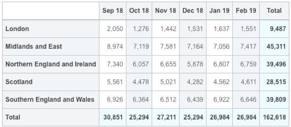
The following six-month rolling report displays a count of transactions grouped by month. Rather than selecting static month values, saved queries with dynamic descriptions have been used to drive the report. This means that when the report is opened next month, the month values will update automatically:

First, six saved queries were created. Each month value is driven by a saved query with the following syntax:

Transaction_Date:["FIRST_DAY_OF_MONTH-6MONTHS" TO "LAST_DAY_OF_MONTH-6MONTHS"]

Simply change the ‘-6MONTHS’ values to ‘-5MONTHS’, ‘-4MONTHS’ etc. to create a number of queries looking at a different month:

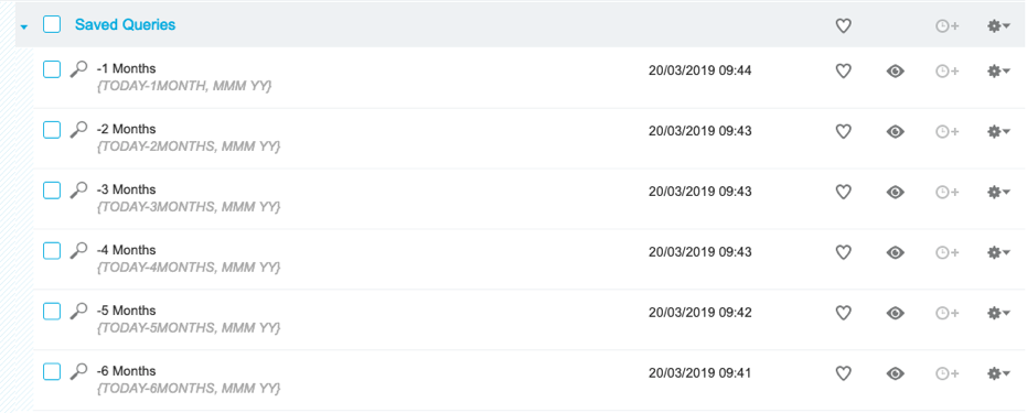
In the above examples, simple dynamic descriptions have also been added for every query.

The report has been created using a single Row and a single Column, with the Saved entry selected, in the Axes tab:

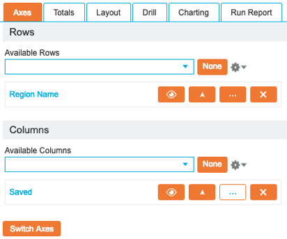
Using the Saved column entry, a number of saved queries can be selected. 

These are loaded into the report using the … icon for the Saved entry:

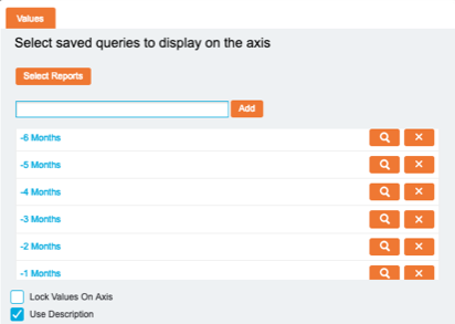
Ensure the Use Description option has been enabled. The report will then refer to the saved query’s dynamic description rather than the static query name. If there is a blank description, the name will be used instead.

With the Total Type set to the default Count option, the report will simply count the records that are returned from each query. The dynamic query syntax ensures that the report will automatically update to reflect a rolling six-month period, negating the requirement to update reports every month.

Dynamic descriptions have the ability to use CASE or IF statements to select different dynamic dates depending on a condition. In this example, we may want to hold off shifting the months forward until working day 2 to allow for more time to review the previous month in full, against the one six months prior.

Use the above CASE statement to replace the description within the -1 Months query to enable this behaviour. Do the same, but adjusting for the number of months, for the subsequent queries.

Note: you will need to add some additional days to the FIRST_WORKING_DAY_OF_MONTH to simulate the first working day before and after your current day of the month. For example, on the 15 Jan 2024 you would use FIRST_WORKING_DAY_OF_MONTH+13DAYS & FIRST_WORKING_DAY_OF_MONTH+14DAYS to test both conditions.

Report Using a Saved Query with Field Comparisons

Saved queries can make use of the same functions available when writing query syntax, the following example compares values between two columns.

Save the following queries run against the EPOS Index:

Single item sales

This report displays the number of sales of a single product per transaction for each region. Using our saved field comparison queries, we are able to show the difference between adjusted and non-adjusted basket values:

The report has been created using a single Row 'Region Name' and a single Column, with the Saved entry selected, in the Axes tab:

With the Total Type set to the default Count option, the report will simply count the records that are returned from each query.

Sales with a discount higher than the basket value

Using our saved field comparison queries, this report displays the number of sales where the discount value is higher than the basket value for each region and by payment method:

The report has been created using Rows with the Saved entry selected (but hidden) and 'Region Name' & 'MOP', in the Axes tab:

With 'No of Transactions' using the Total Type set to the default Count option, the report will simply count the records that are returned from each query. 'Basket Value' & 'Discount Amount' have been selected using the Total Type set to Sum and the corresponding measure selected.

Products sold at a profit or Loss

Using our saved field comparison queries, this report displays the number of sales where products have been sold at profit vs. loss with a grouping hierarchy drillable by Department and Group:

The report has been created using Rows 'Product Department', 'Product Group' and 'Product Name' and a single Column, with the Saved entry selected, in the Axes tab:

With 'No of Transactions' using the Total Type set to the default Count option, the report will simply count the records that are returned from each query. 'Total Average Profit' has been selected, same as previously, using the Total Type set to Average and Line_Price-Cost_Price selected as the calculation.