This guide has been written to outline the steps required to Index, join, shape and flatten data using the Database Wizard, Amalgamated Wizard and ETL Wizard to automate the creation of a customer master record, with the final output summarising customer activity across the business.

To facilitate this level of data processing, the Extract, Transform & Load (ETL) functionality is a vital component. This is due to how CXAIR processes data when Indexed on the system.

When building an Index, CXAIR handles the retrieved data row-by-row. Therefore, there is no grouping at this point and no way to relate rows to each other. For example, the same Customer ID appearing on each row is inconsequential – CXAIR simply stores the rows in the order they are retrieved.

To discover and specify these relationships, these Indexes can then be used in the Crosstab functionality where fields can be grouped at row or column level before aggregated values are derived at run-time. For example, using a date field as a column value will order the values in the report and update the output accordingly.

With this in mind, the following questions pose a problem when simply viewing the raw data: 

When was a customer’s first transaction? What was the value?
What is the total balance value for a single customer across multiple accounts?
What is the most recent transaction value?

The answers to these questions cannot be determined without prior grouping at customer level, as each transaction is stored as a single row.

This is where the ETL functionality and its fundamentally different approach to data processing is crucial, as it is possible to loop through data based on a set of keys to group items together. Using the wizard, a number of grouped aggregations can be written out to the Index that negates the requirement for report-level relationship discovery.

For the purpose of this guide, demonstration data has been used that contains three separate customer, account and transaction tables. For a copy of this sample dataset, please contact Connexica.

Creating the Source Indexes

Three Indexes will be created that each serves a specific purpose, providing key information for an area of the business.

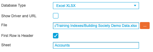
Using the Database Wizard, select Excel XLSX as the Database Type and use the File option to select the supplied Excel file.

For the first Index, enter ‘Accounts’ into the Sheet textbox. For the second Index, repeat the above process and instead enter ‘Customers’ into the Sheet textbox and for the third Index, enter ‘Transactions’ into the Sheet textbox:

Ensure the three Indexes are added into the same Search Engine and the Home screen should resemble the following screenshot:

The Accounts Index contains multiple account information for a single customer:

The Customers Index contains a record per customer, detailing personal information:

The Transactions Index contains transactional-level information for a single customer across multiple accounts:

Amalgamating the Data

With three separate Indexes now created, the Amalgamated Wizard can be used to join the data into a single Amalgamated Index.

This is facilitated by two joins. First, join the Customers and Accounts Indexes using a Left Outer join and select ‘Customer_ID’ as the common field. This will result in account information being added for every customer where the ‘Customer_ID’ field matches.

Leave the Display Fields checkboxes blank to include every column in the resulting output:

Next, create a second join that combines the Accounts and Transactions Indexes using a Left Outer join with ‘Account_Number' used as the first common field. For this join, a second common field is also needed. Click Add Link and select ‘Account_Type’ and ‘Acc_Type’ to meet this requirement. Establishing this second condition ensures that a unique account number is not matched to the wrong type of account.

From the Accounts Index Display Fields, leave the checkboxes empty to bring through every column, while from the Transactions Index, select the ‘Account Name’, ‘Trans ID’, ‘Transaction Date’, ‘Transaction Type’ and ‘Transaction Value’ fields to ensure duplicate fields are not in the output:

Use the Add to Search Engine drop-down list to specify the Search Engine the resulting Index will be added to, enable the Build Now option and click Create to complete the process.

The resulting Index now contains a row for every transaction with the additional customer and account-level columns present: 

Extra Field Calculations

With an Amalgamated Index now created from the three source Indexes, the output can be further supplemented by utilising the Extra Fields functionality. Written at Data Source Group level, calculations can be added that derive additional columns at build-time.

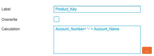
The first extra field that can be added to the Amalgamated Index concatenates the Account Number and Account Name fields to create a composite key called Product Key. This will be used in later stages to denote the number of unique accounts opened by a customer and uses the following logic:

AccountNumber + '-' + AccountName

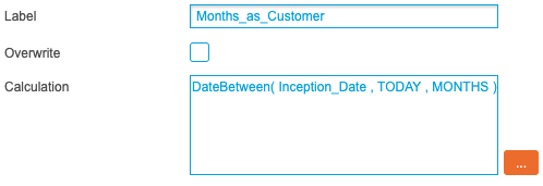
The second extra field, Months as Customer, dynamically compares the Inception Date value for every row and compares it to the current system date. The difference is then written out in months. This uses the following logic:

DateBetween(InceptionDate , TODAY , MONTHS)

Once the two calculated fields have been saved, rebuild the Index and validate the results in the Query screen.

Saved Queries

With rows from multiple accounts joined in a single Index, the following queries can be used to access key areas of interest:

+Account_Status:"Active"
+Account_Status:"Closed"
+Account_Status:"Offer"

These queries provide a cohort of data for active and closed accounts, along with any accounts that have been offered to a customer. Save these queries to utilise this dynamic filtering when creating aggregations in the ETL Wizard.

ETL Processing

In this example, the data processing is split into five distinct stages in order to shape the data into the final output.

Using the ETL Wizard, select the previously created Amalgamated Index from the Index drop-down list to reveal the necessary processing options. (The ETL Wizard allows additional steps to be added directly within the ETL to create these Database & Amalgamated Indexes. Clicking the '+' plus button lists these optional steps.)

Stage 1

The first stage will flag the first and last transaction for each customer and will count their number of accounts, products and transactions.

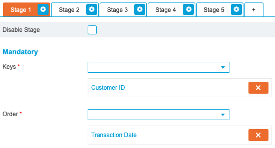
When using the ETL Wizard, each stage requires a Primary Key value entered in the Key drop-down list, and a field that will be used to order the output entered in the Order drop-down list.

As the output will be based at a customer-level, select ‘Customer ID’ from the Key drop-down list. Select ‘Transaction Date’ from the Order drop-down list to specify that the data will be ordered by the date of each transaction:

From the Flags tab, select the ‘Transaction Date’ field from the Is First Minimum and Is Last Maximum drop-down lists. This will identify the first and last transaction date for each customer:

In the Aggregations tab, use the Count Unique option to count the number of accounts, products and transactions for each customer. This is achieved by selecting a key field that denotes each area of interest. Select ‘Account Number’, ‘Product Key’ and ‘Trans ID’.

Additionally, select the ‘Transaction Value’ field from the Sum drop-down list to sum the values from multiple rows:

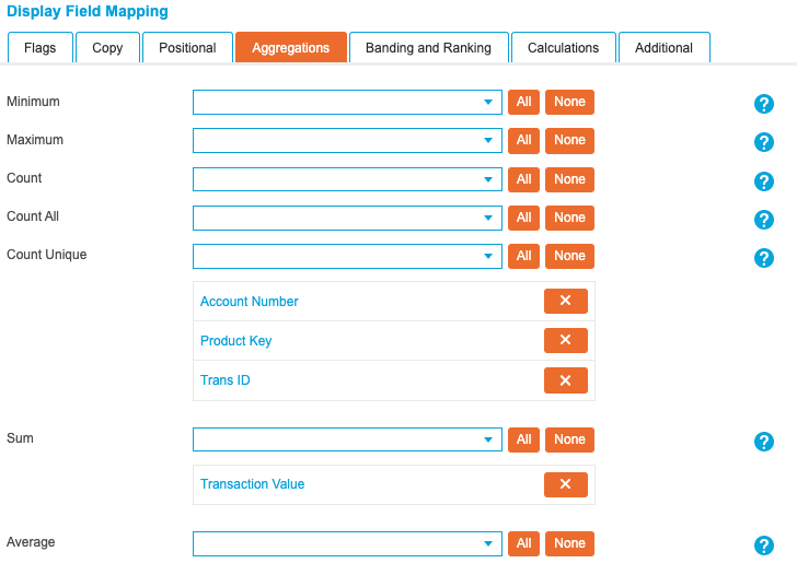
As the Is First Minimum and Is Last Maximum flags have been set, the Additional tab provides further options to tailor the output when the flag is true. Set the ‘Account Type’ and ‘Transaction Date’ fields for the first transaction, and the ‘Transaction Date’, ‘Transaction Type’ and ‘Transaction Value’ fields for the last transaction:

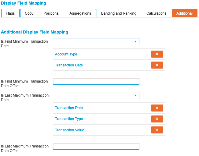
By setting these options in the Additional tab, each customer’s first transaction is flagged and the account type is added to the row. Additionally, each customer’s last transaction is also supplemented with the date, type of transaction and the value of the transaction.

Stage 2

The next three stages all perform the same actions against different subsets of data, each pertaining to a different account type. 

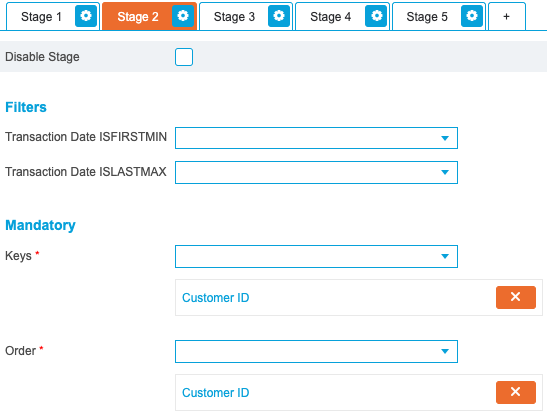
The second stage will count closed products per customer and does not need the data to be output in a particular order. Therefore, select ‘Customer ID’ for both the Key and Order drop-down lists:

In the General section, select the closed accounts query saved previously and enable the Others option:

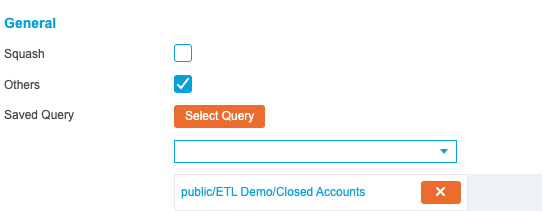
Using a saved query at this point will filter down this stage to rows of interest. Without the Others option enabled, any rows not returned by the saved query are discarded. When enabled, these results are amended to the bottom of the stage output for use in future stages. This means that stages three and four can still utilise other cohorts of data not used in this stage.

From the Aggregations tab, select the ‘Product Key’ field from the Count Unique drop-down list. Due to the added query, this will count the number of closed accounts for each customer:

Stage 3

Repeat the options specified for Stage 2, instead selecting the Active Accounts query. This will count each active account per customer.

Stage 4

Repeat the options specified for Stage 2, instead selecting the Offered Accounts query. This will count each account offer per customer.

Stage 5

The final stage deduplicates records and squashes the data into a single row per customer. This is achieved by selecting ‘Customer ID’ in both the Key and Order drop-down lists and selecting the Squash option:

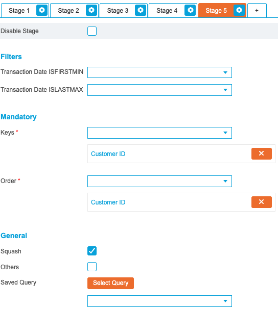
When the Squash option has been enabled, the fields that will be present in the output now need to be specified in the Copy tab.

By default, every field is added to the Copy drop-down list.  However, as the output relies on unique values, remove all entries from the Copy drop-down list and instead populate the Distinct drop-down list with the required fields:

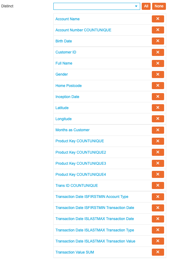
If preferred, these fields can instead be added to the Unique drop-down list at this point, which will perform the same function but order the values. As ordering the values at this point will not provide any meaningful insight, this is not required.

With the all five stages configured, use the Add to Search Engine drop-down list to specify the Search Engine the resulting Index will be added to, enable the Build Now option and click Create to complete the process.

Renaming Key Fields

To enhance the end-user experience and make the fields easier to understand, navigate to the Index level of the created ETL Index and open the Index Fields options.

From here change the text in the Display Field text to better represent the field contents. For example, change ‘Account_Number_COUNTUNIQUE’ to ‘No. of Accounts’.

For a full list of recommended field names, please see the below screenshot:

In the Query screen the Index should now resemble the following screenshot:

This ETL output contains a row per customer, outlining a number of key metrics to provide a view of activity across numerous areas of the business.

Automating the Output

With the data processing now complete, schedules can now be established to automate the entire process and account for new and changed records.

Rather than creating individual schedules for each component, this will be achieved using three Index schedules. The first will rebuild the Indexes from the source Excel sheet, the second will rebuild the subsequent Amalgamated Index and the third will rebuild the ETL Index.

First, navigate to the System Overview screen and select the three source Indexes:

Once selected, click Collections then Save and name the Collection ‘Source Data’. By grouping these three Indexes into one Collection, a single Index schedule can be created that will queue all contained Indexes at build-time, negating the requirement for many Index schedules.

Navigate to the Index Schedules screen and click New. Enter ‘Source Indexes’ into the Name textbox and select the ‘Source Data’ collection from the Items drop-down list:

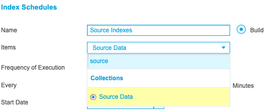
Use the Frequency of Execution drop-down list to specify how often the schedule will run and click Create Schedule to complete the process.

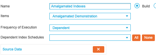
Next, create a new schedule called ‘Amalgamated Indexes’ and add the previously created Amalgamated Index using the Items drop-down list. From the Frequency of Execution drop-down list, select Dependent. This allows the schedule to only run once another schedule has completed, ensuring that the Index does not build until all of the source data has been refreshed successfully. Select the ‘Source Data’ schedule from the Dependent Index Schedules drop-down list and the screen should resemble the following screenshot:

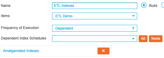
Finally, create a third schedule titled ‘ETL Indexes’ and select the previously created ETL Index selected from the Items drop-down list and Dependent from the Frequency of Execution drop-down list. This time select the ‘Amalgamated Indexes’ schedule. This will instruct the system to only perform the ETL processing once the Amalgamated Index has built. The screen should resemble the following screenshot:

With all three items created, the following schedules should be visible:

Creating these dependent schedules will guarantee that the Indexes automatically build in the correct order, accounting for new information and changed records over time.